There are many applications for taking fourier transforms of images (noise filtering, searching for small structures in diffuse galaxies, etc.). I wanted to point out some of the python capabilities that I have found useful in my particular application, which is to calculate the power spectrum of an image (for later separation of the distribution of stars from the PSF and the noise; see Sheehy et al. 2006).
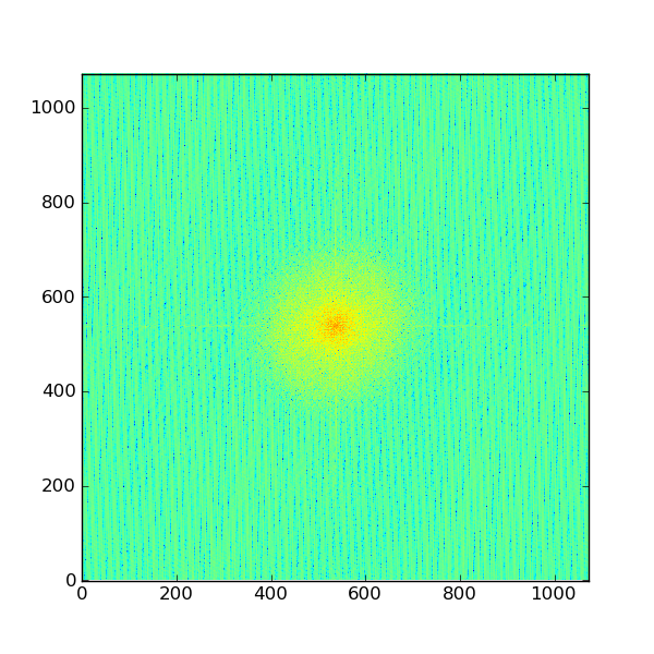
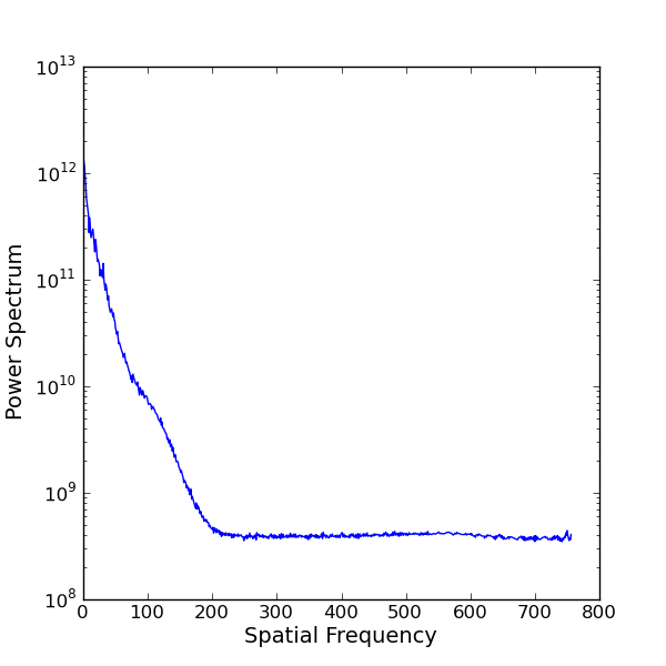
Below I have posted an example snippet of code, which you can also find on the wiki. But first, some figures to show what we are doing — an astronomical image (left), the 2D power spectrum of the image (middle), and the azimuthally averaged 1D power spectrum (right).

The bulk of the heavy lifting can be done using SciPy’s fftpack. I also wrote radialProfile.py and it is very crude at the moment.
[code lang=”python”] from scipy import fftpack
import pyfits
import numpy as np
import pylab as py
import radialProfile
image = pyfits.getdata(‘myimage.fits’)
# Take the fourier transform of the image.
F1 = fftpack.fft2(image)
# Now shift the quadrants around so that low spatial frequencies are in
# the center of the 2D fourier transformed image.
F2 = fftpack.fftshift( F1 )
# Calculate a 2D power spectrum
psd2D = np.abs( F2 )**2
# Calculate the azimuthally averaged 1D power spectrum
psd1D = radialProfile.azimuthalAverage(psd2D)
# Now plot up both
py.figure(1)
py.clf()
py.imshow( np.log10( image ), cmap=py.cm.Greys)
py.figure(2)
py.clf()
py.imshow( np.log10( psf2D ))
py.figure(3)
py.clf()
py.semilogy( psf1D )
py.xlabel(‘Spatial Frequency’)
py.ylabel(‘Power Spectrum’)
py.show()
[/code]
If you have suggestions for the above examples or other related code snippets or helper functions, let me know or comment below. I have posted this example on the wiki and will keep it updated with your suggestions.
Thanks for the nice recipe. Do you use it for PSF reconstruction? If so, could you please give us more details on that? Practical implications are really interesting here…
I’ve been working on very similar code: http://code.google.com/p/agpy/source/browse/trunk/agpy/psds.py. It uses numpy’s fft if scipy fails. The tricky bit you left out of the example, though, is getting the spatial frequency in the right units.
It looks like the power spectrum has a shoulder at freq=100. What is causing that? If the PSF were Gaussian, then the power spectrum would also be Gaussian.
This is an adaptive optics image, so we have approximately a diffraction limited core + seeing halo. So at those intermediate frequencies, you are seeing the AO correction.
Adam, you hit the nail on the head. I know you can use fftfreq to construct the spatial frequencies, but I just haven’t gotten around to constructing the proper 1D X and Y (or nu_x and nu_y) axes or a 2D meshgrid. Thanks for the example! Would you be interested in sharing your code (or a link to it) on the wiki and if so, can you give me a brief example of how you use it?
Ivan, right now I am applying the Sheehy et al. method to derive an aperture correction for crowded field adaptive optics photometery (1D PSF estimation from image + known positions of stars + model of atmosphere/AO system/telescope). Currently their code is in IDL, so I have been using python to call out to idl (via pIDLy). I wanted to explore whether it would be worth porting the code to python; especially since I was contemplating whether the code could be expanded to 2D. However, I think a more productive direction would be the methods/code in the papers by Matthew Britton (use empirical PSF from somewhere in an image + Cn2 profile of atmosphere to reconstruct the PSF at all other points in the image). I am using laser guide star AO with an off-axis tip-tilt star so this complicates things enormously.
Roy, this is just a background noise causes the constant term, check e.g. eq. 6-7 in Sheehy et al. 2006.
Jessica, thanks for your comments. I’m after another problem actually: very crowded field photometry. Seems that I have no chance to estimate PSF from the image itself, so I’m exploring what FT can give here…
Sure thing. I have test code + a test image:
http://code.google.com/p/agpy/source/browse/trunk/tests/
http://code.google.com/p/agpy/source/browse/trunk/tests/example_psd.py
http://code.google.com/p/agpy/source/browse/trunk/tests/PSF.fits
The example shows the power spectrum of a non-Gaussian PSF with sidelobes that should approximately correspond to Airy rings. I don’t bother with the 2d PSD (even though the code is written for that) because I don’t really use PSDs.
Ivan: The autocorrelation (rather than the PSD) should contain information about the psf, I think. Though when I tried it myself it looks like the autocorrelation^2 has ~the same FWHM… I’m not sure exactly why that should be.
A few years back I wrote a routine similar to your “radialProfile” that computes average, mean, min/max in annuli of an image, with the option to define the image coordinate system (and thus the center-of-interest). If anyone wants to take a look, I’ve put it online here.
For a centered image, the syntax is just:
import pylab as py

from radial_data import radial_data

data = radial_data(image, annulus_width=2, rmax=100)

py.plot(data.r, data.mean)
The tricks you used in radialProfile.py are much faster than the not-so-clever tricks I used in my PSD code. However, it excluded inner & outer points, and I wanted the standard deviation too…. so modified code is posted at the wiki and agpy.
Thank you very much. In radialProfile.py line 17 instead of
center = np.array([(x.max()-x.min())/2.0, (x.max()-x.min())/2.0])
should read
center = np.array([(x.max()-x.min())/2.0, (y.max()-y.min())/2.0])
in my opinion!
@Adam: i did try your code prior to this one, but it has many more dependencies (like pyfits), which aren’t really necessary for psd, imho.
Omar – Yes, the agpy package has a lot of extra requirements… it’s not really packaged for distribution at the moment. However, the PSD and radialprofile codes should stand on their own. Would it be helpful if I packaged them separately? If so, I’ll work on that.
One thing to note – the radial profile code included in the above post, and that I had previously used, is very slow for large images. There are some nifty tricks using numpy.histogram to make it faster. I’ve implemented them here:
http://code.google.com/p/agpy/source/browse/trunk/agpy/radialprofile.py
but in short, the fast way to make the radial profile, once you’ve made a “radius” array and determined the bin locatinos, is:
np.histogram(r, bins, weights=image)
@Adam: the problem was, when i import agpy.psds python would try to parse agpy.__init__ and that includes all the dependencies.
if i might wish me a pony: scipy.fftpack might actually need a psd function, so i would say this is something you might want to suggest to scipy for inclusion!
Omar: I looked into this, but apparently the process is to make a “scikit” first. I’ll look into doing that, but not immediately.
In the meantime, I’ve split up agpy into some sub-packages. You should now be able to access PSDs without any unnecessary dependencies from the module AG_fft_tools.
Hello,
Ok I am new to this and I would love to use this to make powerspectra of extinction maps I have. However, in order to compare, I would need to know how to convert this to a spatial wavelength. Right now I cannot make heads or tails from the spectra I’m getting.
I would like to compare directly to the plots in Combes et al 2012. But to do so, I need to know what point in the plot corresponds to one pixel and what to the size of the image.
help would be greatly appreciated!
Benne
I have NOT been able to find the issue here, does anyone know what may be happening?
thanks in advance,
*************
Traceback (most recent call last):
File “fftimg.py”, line 19, in
psd1D = radialProfile.azimuthalAverage(psd2D)
File “/home/jdiazama/FFT/radialProfile.py”, line 14, in azimuthalAverage
y, x = np.indices(image.shape)
ValueError: too many values to unpack
**********
Hi!
I found a small typo, just FYI
psd2D = np.abs(F)**2
Code is very helpful, thanks!!!!
@Jessica & @Adam: Thanks for the code and explanations! I am trying to use it for a non astronomy related project, which is to measure the typical distance between patches of vegetation in arid areas. I have areal images of areas and I want to extract the power spectra of those images, such that I know if there is a pick at a certain wavenumber.
I wanted to ask, in order to have the correct wavelength, I need to let the code know what is the size and resolution of the image, don’t I ? Where should this part be in the code?
Thanks Jessica, your code was very helpful 🙂
Hi, thanks for your code, I try to use it in a different context than astronomy – in finding typical distances between vegetation patches in dryland ecological systems. I have difficult though to detect a typical distance of a rather simple pattern – stripes of a given wavenumber. I’ve written a Jupyter notebook that I uploaded to Github repository here –
https://github.com/Omer80/transform_stripes_to_hexagons
But in general – how do you detect the values of the highest peaks in psd1D ?
Hi Jessica
A related question. If you have a series of astronomical images taken in space such as by the SOHO telescope, what FFT technique would you use to filter out comets that are at or near the noise level of the image. Is it possible to filter out a small (say 1-2 pixels wide) faint comet from a series of such images using FFT?
Thanks Peter