Katharina Lutz is a postdoc at the Centre de Données astronomiques de Strasbourg (CDS). She works on gas and star formation in nearby galaxies, and the dissemination of the Virtual Observatory (VO) and the CDS services. This involves maintaining and developing tutorials, and mentoring at VO Schools. This post is the second in a series of articles on services offered by the CDS, and was written in collaboration with the CDS Python developers, who are currently working on further MOCpy and astroquery developments, and the CDS dissemination team, who are preparing for the next VO training events.
Welcome back to our mini-series about Python access to CDS services. In our first post, we introduced ipyaladin, a convenient way to visualise your favorite sources. In this second post, we move on to the one question that every observational astronomer asks all of the time: which surveys have observed this object?
At the CDS, we have developed Multi-Order Coverage (MOC, an IVOA standard) maps to help you answer this question. A MOC describes the footprint of a survey or, in more technical terms, it is a map (or list) of all of those HEALPix cells (to a chosen resolution) that are covered by a survey. MOCs use the HEALPix tessellation and are thus an efficient way of describing the complex footprints of surveys on the sky as well as arbitrary polygons from a list of sky coordinates, or the sky coverage of catalogues. Furthermore, they allow for the calculation of intersections and unions of these patches on the sky to be performed quickly and efficiently. Recently, the MOC concept has been extended beyond the description of spatial coverage on the sky to also encode the coverage of a dataset in time (Space and Time or ST-MOCs describing when and where data were taken, IVOA standard in progress).
The CDS MOC server, which provides MOCs for all datasets that are available through the Virtual Observatory, can be queried with the cds package in astroquery. Using the MOCpy package, you can furthermore create MOCs of your own datasets.
Now how can this facilitate your research? Consider the following use case: from a catalogue of sources you would like to select those objects that have been observed both with GALEX and HST, and are located at low Galactic extinction. To do so, you could download the MOC of GALEX and HST and get the intersection of the two (the result is shown in Figure 1). Depending on your internet connection, that should only take you a few seconds. In the next step, you create a MOC from a Galactic extinction map but tell MOCpy to only include those pixels that have a certain pixel value. Once you have described a region of interest on the sky with a MOC, catalogues can be filtered with one single line of Python code in order to select sources that have sky positions within the MOC.
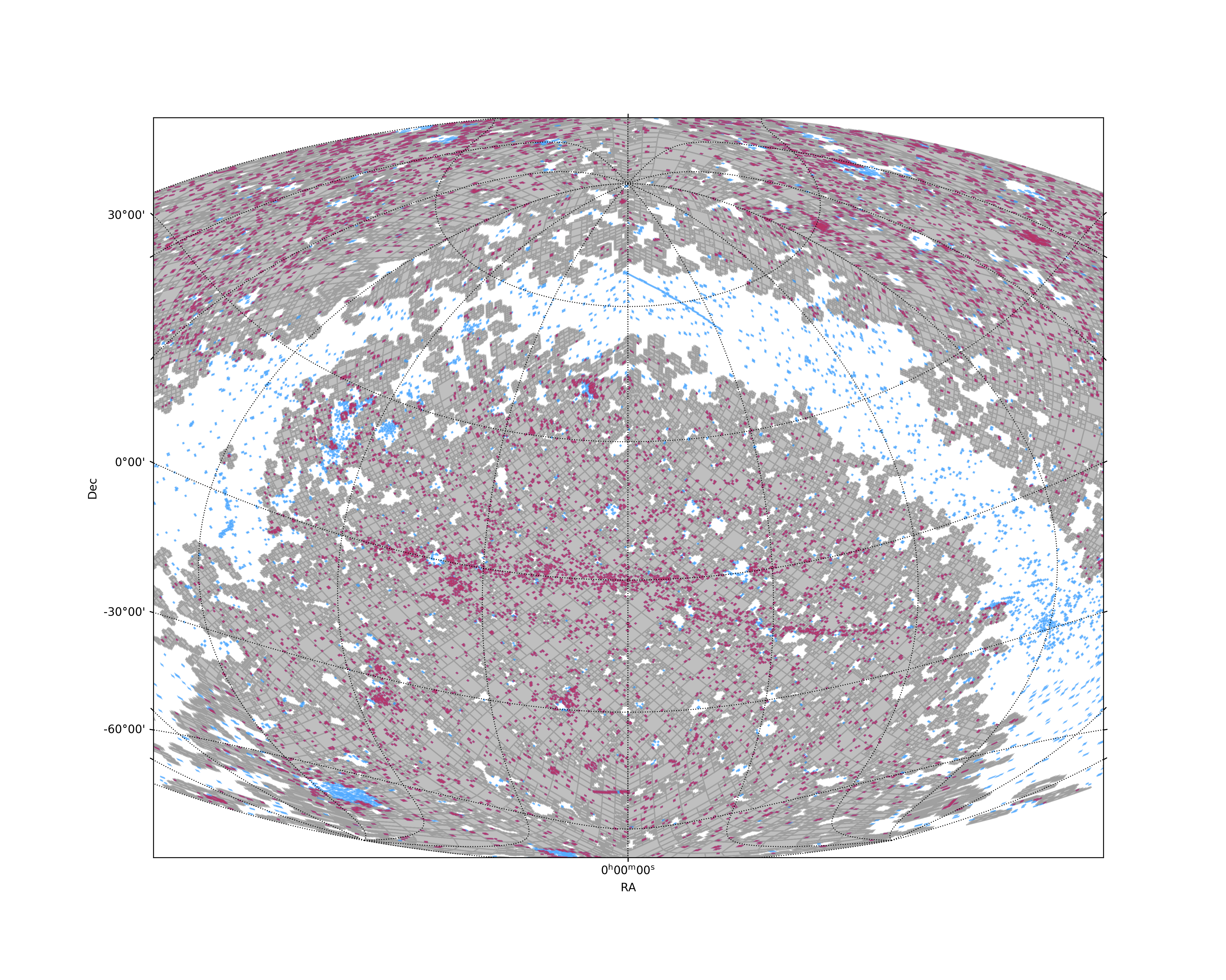
Figure 1. The MOC of the Galex footprint (grey), all HST observations (blue), and their intersection (red) visualised with MOCpy.
For visualising MOCs or catalogue tables on the sky, you can either plot the MOC with MOCpy utilising Astropy’s WCS axes in matplotlib (Figure 1), or use the ipyaladin widget.
If you would like to have a look at a few tutorials we assembled, hop over to GitHub or try it with your own data. Tell us how it works for you and contact our helpdesk for questions. We also welcome issues on GitHub and are on Twitter, Facebook and YouTube.